On GPU programming:
Hello!
Hello and welcome to my first blog ever. Today, and for the next couple of weeks, we are going to talk about GPU programming using CUDA C++.
Setup
CUDA (Compute Unified Device Architecture) is a GPU programming platform developed by NVIDIA (the GPU company you've probably already heard of). To get to what CUDA is, how it came about, and how you can use it to make your programs run faster, we need to establish some other information.
Introduction
Early computers had only single processor we call the Central Processing Unit(CPU). These CPUs from back then right up to now are relatively good at handling complicated control flow, sequential dependency, and high precision computations. However, the scientific computing world has an insatiable desire for performance. As we have figured out over the last couple of decades with the demise of Dennard Scaling and Moore's law (the death of Moore's Law is somewhat of a controversial topic with many claiming that it is already dead, while several well known names in the computing world including Jim Keller and Peter Lee making hilarious jokes[9:04] about how it is not Moore's law that is dead, but rather that the number of people predicting the death of Moore's law doubled every year). Several computer architects from way back then had already identified that such scaling would not go on forever and so naturally computer architects (literally in the 60s) identified parallelism as the way to go forward. Although such disregard for the single processor approach was not met without skepticism with one of the more notable skeptics being Gene Amadahl, who noted in his 1967 paper (which described what is now known as Amadahl's law) that there is a limit to the performance increase one can obtain by making an algorithm parallel (running it on parallel cores). This was because of the sequential dependence that naturally arises in virtually all computer programs. Ever since then, the world, particularly the scientific computing world has changed. We have shifted on to what we call today as heterogeneous computing systems which combines one or more CPUs with accelerator devices like GPUs and even more recently TPUs. GPUs by themselves are not new phenomenon. Their existence goes right back to the 60s. Traditional GPU pipelines consisted of programmable vertex processors that executed vertex shader programs and pixel fragment processors that executed pixel shader programs. GPUs back then were not really programmable for scientific computing meaning scientists either had to rely on domain experts of computer graphics or learn OpenGL and shaders themselves to get anything done. Now, anyone that has written a line of OpenGL code knows it is not fun to deal with. And this takes us back to CUDA.
A typical CPU-GPU configuration may look like either of the following.
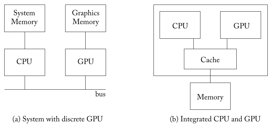
Fig: General Purpose Graphics Processor Architecture (Aamodt et. al)
Emergence of CUDA
In their landmark whitepaper for the Tesla architecture NVIDIA introduced a unification of vertex and pixel shaders with their extension in what they called a Compute Unified Device Architecture (CUDA). With this unification came a new modern parallel programming model. GPUs supporting this architecture could be programmed using the CUDA parallel programming model on top of the same old C programming language slightly extended.
CUDA programming model:
The architecture of CUDA (down below at the hardware level) is SIMD. If you are writing a vertex shader program, you write it for one thread describing how it should process a vertex. Similarly, when you write a CUDA kernel, you describe the behavior of a single thread and the CUDA compiler and the runtime will handle the complicated balancing and synchronizing for you.The kernel is the code that you write on the CPU (we call it the host device in almost all heterogeneous computing configurations) but runs on the GPU (we call it just the 'device').
CUDA threads and SIMT
In CUDA, threads are grouped into blocks and blocks are themselves grouped onto a grid. A grid can be three dimensional, consisting of multiple blocks each of which can be three dimensional and contains threads along each dimension. All the threads of the same thread block are executed on the same Streaming Multiprocessor (we are not going to get into the nifty details of the graphics architecture in this blog). Threads are a logical construct and the threads in a block can communicate because they share the same shared memory on a streaming multiprocessor. It is because of this separation of threads, blocks and grid that makes CUDA scalable to a multitude of different types of GPUs.
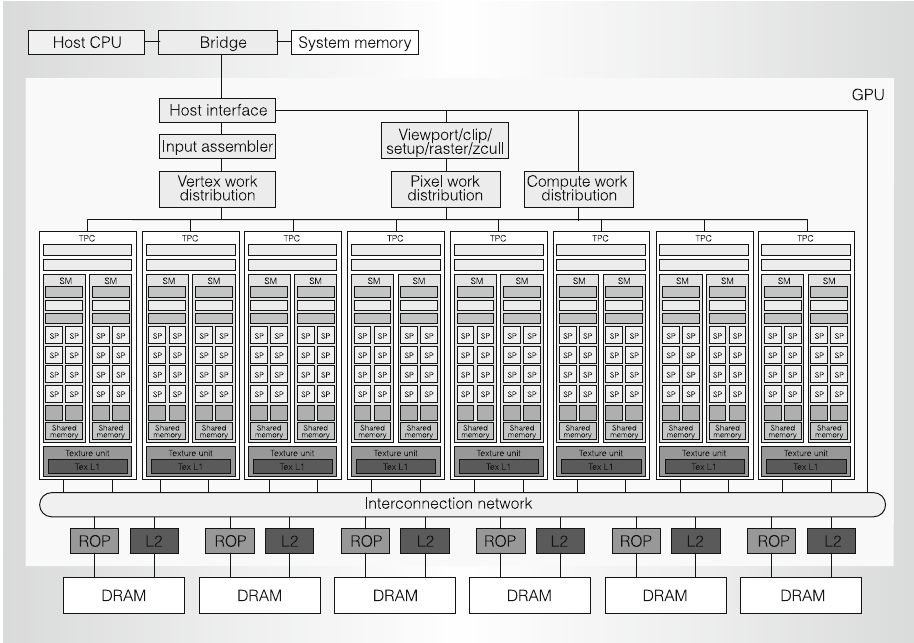
Fig: from NVIDIA's original Tesla architecture whitepaper, featuring multiple SMs with their own SP's and so on.
CUDA workflow:
A common workflow when using CUDA goes something like this:
You initialize your data in the CPU (host memory) and then perform
cudaMemcpyto send the data to the GPU.
You call your GPU kernel with this GPU data
You copy back the data (processed) from the GPU memory to CPU memory.
We've talked enough about the CUDA thread hierarchy, so I suppose we should move on to memory hierarchy.
The GPU consists of a shared memory space and a global memory space. Global memory is analogous to the CPU DRAM memory, while shared memory is more similar to CPU cache. Unlike the CPU cache however, GPU shared memory can be controlled by the user. In fact the same applies to GPU threads as well. CPU threads can be a menace to synchronize, but CUDA threads are far easier to handle and there are just more constructs for helping us handle them.
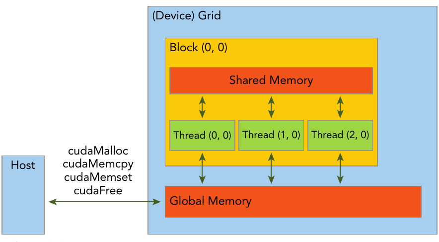
Fig: dislaying memory hierarchy taken from Professional CUDA C Programming (Cheng et al.).
In a heterogeneous computing system, the CPU memory and GPU memory are normally separated by a PCI-Express bus and so, this separation of memory seems natural. However, CUDA also gives us a unification of these two memory spaces, called Unified Memory so you don't need separate pointers to CPU and GPU memory in your code.
Getting Started writing CUDA Kernels
First you would want to have CUDA installed on your device if you have an NVIDIA graphics card. Go to unix shell and just do
which nvccIf you get something like
/usr/local/cuda-11.7/bin/nvcc
then congrats, you have cuda installed in your computer and you're good to go. To really use CUDA efficiently you need to master the thread hierarchy, the memory hierarchy and the barrier synchronization capabilities that the CUDA api provides.
Writing a simple vector additon routine on the CPU.
void add_vecs_on_cpu(float* C, float* A, float* B, size_t n) {
    for (int i = 0; i < n; ++i) {
        C[i] = A[i] + B[i];
    }
}

int main() {
  int n = 1024;
  int nbytes = N * sizeof(float);
  float* h_a = (float*)malloc(nbytes);
  float* h_b = (float*)malloc(nbytes);
  float* h_c = (float*)malloc(nbytes);
  //set the arrays to some value.
  for (int i = 0; i < n; ++i) {
      h_a[i] = 1.f;
      h_b[i] = 2.f;
  }
  //add them on the cpu
  add_vecs_on_cpu(h_c, h_a, h_b, n);
  //print them all
  for (int i = 0; i < n; ++i) {
      printf("%f\n", h_c[i]);
  }
  printf("printing on the cpu over\n");
}
This was easy, now let's write a CUDA kernel 'add_vecs_on_gpu'.
__global__ void add_vecs_on_gpu(float* C, float* A, float* B, size_t n) {
    int ix = blockIdx.x * blockDim.x + threadIdx.x;
    if (ix < n) {
        C[ix] = A[ix] + B[ix];
    }
}

int main() {
  int tpb = 256;//threads per block
  int n = 1024; //total no. of elements in the flat array
  int nbytes = N * sizeof(float);
  //pointers to device memory
  float* d_a;
  float* d_b;
  float* d_c;
  //arrays on the host
  //allocate N * sizeof(float) elements
  float* h_a = (float*)malloc(nbytes);
  float* h_b = (float*)malloc(nbytes);
  float* h_c = (float*)malloc(nbytes);
  //arrays on the device
  //allocate n * sizeof(float) elements on the device
  cudaMalloc((float**)&d_a, nbytes);
  cudaMalloc((float**)&d_b, nbytes);
  cudaMalloc((float**)&d_c, nbytes);
  //set the arrays to some value.
  for (int i = 0; i < n; ++i) {
      h_a[i] = 1.f;
      h_b[i] = 2.f;
  }
  cudaMemcpy(d_a, h_a, nbytes, cudaMemcpyHostToDevice);
  cudaMemcpy(d_b, h_b, nbytes, cudaMemcpyHostToDevice);
  add_vecs_on_cpu(h_c, h_a, h_b, n);
  //display
  for (int i = 0; i < n; ++i) {
      printf("%f\n", h_c[i]);
  }
  printf("printing on the cpu over\n");
  //set h_c back to 0.0f to again do the computation on the gpu.
  memset(h_c, 0.0f, nbytes);
  //dim3 = 3 unsigned ints, this defines dimension across
  //x, y, and z, single value means only x
  dim3 blocks(tpb); //no of threads in a block.
  dim3 grid ((n + tpb - 1)/tpb); //no of blocks in the grid
  add_vecs_on_gpu<<<grid, blocks>>>(d_c, d_a, d_b, n);
  //copy the result back to host for displaying
  cudaMemcpy(h_c, d_c, nbytes, cudaMemcpyDeviceToHost);
  //print the result
  for (int i = 0; i < n; ++i) {
      printf("%f\n", h_c[i]);
  }
  //free all allocations
  cudaFree(d_a);
  cudaFree(d_b);
  cudaFree(d_c);
  free(h_a);
  free(h_b);
  free(h_c);
}
Here, global is a CUDA keyword and it indicates that the kernel function will be called from the host and run on the GPU.
Now, due to physical limitations, a block can only have a certain number of threads. In modern GPUs, the limit is something like 1024 threads per block at a maximum. We prefer setting threads per block (tpb) to just 256 for now. After we only have a grid with blocks along a single dimension and blocks with threads along a single dimension for now.
The line
int ix = blockIdx.x * blockDim.x + threadIdx.x;
really just tells each thread what indices of the array it should work on. To find out the 3rd thread of the second block, you need to go past the 1st block across all of its thread (blockIdx.x * blockDim.x) and add the thread id of that thread for that block(blockIdx.x * blockDim.x + threadIdx.x). When we call the kernel like this:
add_vecs_on_gpu<<<grid, blocks>>>(...)
We specify the number of blocks in a grid and the number of threads in a block, i.e. 'grid' variable stores the number of blocks across its 3 dimensions (if .y and .z are unspecified, they are defaulted to 1) and 'blocks' variable stores the number of threads across its 3 dimensions.
We pick a thread per block number of 256, and use that to compute the number of blocks that we need in the line
dim3 blocks(tpb); //no of threads in a block.
dim3 grid ((n + tpb - 1)/tpb); //no of blocks in the grid
The second line gives us the number of blocks we need. instead of
we could also use ceil as in
dim3 grid (ceil(n / tpb)).
This is to handle the case when the total number of elements is not an integer multiple of the number of threads per block.
In the kernel code, we use the if statement to ensure we are not indexing the arrays at indices at which they are not even allocated because if using ceil we are describing an extra block with some unused threads, we don't want those threads to be indexing into the arrays.
CUDA Error Checking
We think of two types of CUDA errors–synchronous errors and asynchronous errors.
Synchronous Errors : Synchronous error is something the host thread knows before launching the kernel code, for example, if the block, and grid dimension are illegal or invalid. It is quite simple to handle such errors.
Asynchronous Errors : All kernel launches in CUDA are asynchronous. This means that the moment you launch the host code reaches the kernel code and no synchronous error is met, the kernel threads are launched on the gpu and the control goes back to the host immediately while the gpu code runs asynchronously. This means that we can't simply use cuda runtime error handling functions in the host code because the error may occur during the runtime of the GPU code a while later. A simple solution to this problem would be to explicitly synchronize the kernel thread so that the handle of control goes back to host code only after all gpu threads have finished executing. For this, one would use 'cudaDeviceSynchronize' and other synchronization calls. Such explicit synchronization is not particularly good for performance and is never tried in production level code. So, for checking asynchronous errors, use synchronization and runtime error capturing API calls like cudaGetLastError and disable all synchronization in production code. A better explanation of error handling in CUDA is described in Lei Mao's blog. Lei is more of an expert on CUDA than I am (well, I am literally just a beginner), so you should really check him out.
For error handling, we define the following macro:
#define CHECK_CUDA_ERROR(val) check_cuda_error((val), #val, __FILE__, __LINE__)

template <typename T>
void check_cuda_error(
                T err,
                const char* const func,
                const char* const file,
                const int line
    )
{
  if (err != cudaSuccess) {
    fprintf(stderr, "cuda error in file: %s at line: %d\n", file, line);
    fprintf(stderr, "Error message: %s %s\n", cudaGetErrorString(err), func);
  }
}
Every time we call cudaMalloc or something, we will wrap it in CHECK_CUDA_ERROR macro from now on.
At this point, you should be able to write your own matrix multiplication kernel in CUDA C++. It should be mentioned however that you should pretty much never write your own matrix multiplication kernel as part of production code because heavily optimized libraries like cuBLAS exist for that already. One will only ever have to write GPU kernels for code that hasn't already been written and optimized or for new research.
Scientific computing and performance metrics of the GPU
Enough CUDA for now, let's get back to some of the challenges in scientific computing with GPUs.
Due to GPUs and massively parallel computing, performance of most scientific code today is not bounded by the speed of computations( even though the GPUs are relatively slow at processing single data, they process a large number of data at the same time), but rather they are bounded by memory access times. To measure this discrepancy in peak computational performance for and memory bandwidth, we simply take their ratio and multiply by the number of bytes of a number (in 64 bit systems this is 8). The peak computational performance is measured in GFlops/s while memory bandwidth is measured in GB/s.
From C++ to Julia
We had a look at what GPU programming in C++ using CUDA looks like. Writing kernels in C++ is hectic as you saw just from the above very simple example of writing vector addition.
This brings us to Julia which is a just-in-time compiled high level garbage collected programming language. We'll use CUDA.jl in julia for the next couple of examples and over the next couple of blogs, all of our work will be in Julia.
Now, there are some really good reasons as to why you should use Julia for GPU programming for scientific work. One is that we don't have to manually allocate and free host and device memory and copy the data with complicated looking functions. The CUDA.jl API for makes the entire workflow really smooth.
The other reason being that despite such ease of use we really don't lose much on performance. It is well documented that a reasonably optimized Julia code can match C++ or even Fortran level performnaces. Another big reason for Julia is the fact that we can write generic GPU kernels.
In C++, (I'm not writing this with any certainty, I am only just beginning to learn CUDA so educate me if I'm wrong), you really can't write generic kernels because the kernel code needs to be compiled with specific type at compile time and so you need to manually template instantiate functions when calling them. This means, you need to specify the types with which the function is called. This is not really very dynamic is it? Well, Julia functions are Just-In-Time compiled. That means, the called function is compiled at runtime with the most specific permutation of types that are passed as arguments (this is done by method table lookup at runtime for all types in the argument list). This is called multiple dispatch. Since at runtime julia knows the type with which the function is being called, it can generate an optimized LLVM IR even for the CUDA kernel code. This makes the process of writing CUDA kernels work for all the different types and also writing code in a dynamic way more fun.
A Simple Exercise In Julia
Let us write a cuda kernel that copies matrix A to matrix B and we shall do some simple performance analysis of our code to get you a feel of what GPU programming looks like in Julia.
using CUDA
using BenchmarkTools

const THREADS_PER_BLOCK = 256
# here, we won't bother checking sizes and so on
function mycopy!(A, B)
    ix = ((blockIdx().x-1)*blockDim().x) + threadIdx().x
    iy = ((blockIdx().y-1)*blockDim().y) + threadIdx().y
    if ix <= size(A)[1] && iy <= size(B)[2]
        @inbounds A[ix, iy] = B[ix, iy] #don't do bounds checking
    end
    return
end
#set matrix size 1000 X 1000
nx = 1000
ny = 1000
threads = 10, 10, 1
blocks = ceil(Int64, nx / threads[1]), ceil(Int64, ny / threads[2]), 1
A = CUDA.fill(1.0f0, nx, ny)
#print(A)
B = CUDA.fill(0.0f0, nx, ny)
#print(B)
@benchmark CUDA.@sync @cuda threads=$threads blocks=$blocks mycopy!($A, $B)
#elapsedtime = @belapsed CUDA.@sync @cuda threads=$threads blocks=$blocks mycopy!($A, $B)
#CUDA.@sync @cuda threads=threads blocks=blocks mycopy!(A, B)
#print(A)
BenchmarkTools.Trial: 10000 samples with 1 evaluation.
Range (min … max): 119.640 μs … 905.558 μs ┊ GC (min … max): 0.00% … 0.00%
Time (median): 121.335 μs ┊ GC (median): 0.00%
Time (mean ± σ): 122.839 μs ± 20.750 μs ┊ GC (mean ± σ): 0.00% ± 0.00%
▁▄▇█▇▆▅▆▆▆▇▇▅▄▃▂▂▁▁▁▁▁ ▂
▇██████████████████████████▇▇▇▇▇▆▇▇▆▇▇▅▆▆▅▆▅▅▆▄▅▅▅▄▅▅▄▄▅▄▅▄▃▄ █
120 μs Histogram: log(frequency) by time 133 μs <
Memory estimate: 256 bytes, allocs estimate: 3.We are copying a 1000 by 1000 matrix within 150 microseconds. Let's do some back of the envelope computations.
Suppose you have an 'nx' by 'ny' matrix and you want to copy it to another 'nx' by 'ny' matrix. This requires nx * ny reads and then nx*ny writes as in the line :
A[ix, iy] = B[ix, iy]
What this line is doing is it is looking for all nx * ny elements of array B in the global memory space of the GPU (this is in global memory because we have done nothing to ensure we are storing and accessing data in the shared memory of respective SMs) and writing all of those values to A in the global memory which is again done for nx*ny times. So, we have a total of memory accesses of Float32 data. That would be a total of GB of data transferred. To compute the total memory throughput, we divide by the minimum elapsed time of the taken time samples. So, in the code, we need to use @belapsed instead of @benchmark macro. We got belapsed to be 0.000117577 in my computer.
So, the memory throughput is :
elapsed_time = 0.000117577
throughput = 2 * 1000 * 1000 * sizeof(Float32) / (10^9 * elapsedtime)68.04051812854554A look at the future:
I guess this is it for today's blog. I just wanted to cover all the simple basics of GPU programming. It's going to take me a while to write another blog, however the next one is also going to be about the GPU programming model with sample code in both C++ and Julia. Till then, stay tuned!